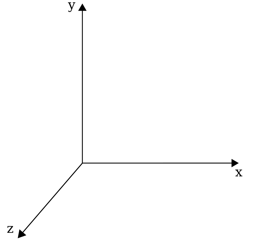
Theory of Dimensionless Products: On Vector Space

On Vector Space

The idea of using ordered pairs to locate points in a plane or ordered triple for points in 3D can be traced back to the mid-17th century.

There are various representation (or definitions) of vector

as directed line segment (arrow)
as arrow with rectangular coordinate system (for 2D but coordinate system in general)
as component of the arrow in the coordinate system. ♻

Notice that these representations introduces geometric properties of a vector. But, representation of vectors as components — coordinate component — makes vectors have a mathematical existence in the sense that the vectors can be analyzed numerically, i.e., analytical or numerical property.

By late 19th century mathematicians concluded that there is "no need to stop at triplets" to define vectors. That is, even if we can no longer extend the vectors geometrically beyond 3D one can analyze vectors as

quadruples of numbers (a₁, a₂, a₃, a₄) for 4D
quintuples of numbers (a₁, a₂, a₃, a₄, a₅) for 5D
⋮

If n is in a positive integer, then an ordered n-tuple is a sequence of n real numbers (a₁, a₂, …, a_n ).
The set { (a₁, a₂, …, a_n), (b₁, b₂, …, b_n), (c₁, c₂, …, c_n), … } of all ordered n-tuples is called n-space and is denoted by ℜⁿ.

Terminologies

ℜⁿ: ordered n-tuples or n-space
ℜ²: ordered pair or 2-space
ℜ³: ordered triples or 3-space

❶

Analytic properties of a vector provides deeper insight

The symbol (a₁, a₂, a₃) in 3-space has two geometric interpretations

as a point with coordinates (a₁, a₂, a₃)
as a vector with components (a₁, a₂, a₃) ♻

In general, (a₁, a₂, …, a_n) in n-space is

a generalized point with coordinates (a₁, a₂, …, a_n)
a generalized vector with components (a₁, a₂, …, a_n)

However, mathematical distinction is unimportant.

In its algebraic form vectors can be denoted using either coordinate notation or matrix notation

For vector u in ℜⁿ its
      coordinate notation is (u₁, u₂, …, u_n)
      matrix notation is
           [u₁, u₂, …, u_n] as row elements
           [u₁, u₂, …, u_n]^T as column elements

If u = (u₁, u₂, …, u_n) and v = (v₁, v₂, …, v_n) are vectors in ℜⁿ then u and v are called equivalent vectors if and only if u₁ = v₁, u₂ = v₂, …, u_n = v_n That is, u = v.

Because of how vectors are defined equivalent implies equal. Therefore, u and v are equal vectors.

❷

Standard operations on ℜⁿ

If k is a scalar, u = (u₁, u₂, …, u_n) and v = (v₁, v₂, …, v_n) are vectors in ℜⁿ the operation u + v = (u₁ + v₁, u₂ + v₂, …, u_n + v_n) is called sum u + v which is a vector in ℜⁿ and the operation ku = ku₁, ku₂, …, ku_n is called scalar multiple ku, also a vector in ℜⁿ.

These operations are called standard operations on ℜⁿ.

Notice that expressed as components operations on large vectors can get unyielding. However, there exist a theorem on the arithmetic properties of the standard operations. The theorem enables manipulating vectors in ℜⁿ without the need of expressing vectors as components.

If k and l are scalars and u = (u₁, u₂, …, u_n), v = (v₁, v₂, …, v_n) and w = (w₁, w₂, …, w_n) are vectors in ℜⁿ then

u + v = v + u Commutative law for addition
u + (v + w) = (u + v) + w Associative law for addition
u + 0 = 0 + u = 0 Adding zero
u + (−u) = 0 ⇒ u − u = 0 Negation law
k(u + v) = ku + kv Distributive multiplication over addition
k(lu) = (kl)u Multiplication by scalar product
(k + l)u = ku + lu Multiplication by scalar sum
1u = u Multiplying one

The arithmetic properties for standard operations of ℜⁿ given by the above theorem applies to vectors represented by either coordinate notation or matrix notation. However the matrix notation is preferred because it is easier to manipulate.

Although it will not be discussed here, there exist another operation, the Euclidean inner product u ⋅ v. Like the arithmetic properties of the standard operations mentioned in the theorem above, the inner product operation is governed by its own set of arithmetic properties.

The n-space ℜⁿ where both the standard operations and the inner product operation is defined is called an Euclidean n-space.

❸

Generalizing Vector Space

The notion of vectors need not be restricted to vectors in n-space, ℜⁿ. One can abstract the most important properties in ℜⁿ such that each property abstracted is considered an axiom. The collection of abstracted properties form a set of axioms.

Notice that the vectors in ℜⁿ automatically satisfy the set of axioms. However, other objects may satisfy the axioms. The class of objects that satisfy the set are the generalized vectors. This new concept of vectors include

old vectors; vectors in ℜⁿ
new vectors; class of objects that satisfy the set of axioms

Suppose k and l are scalar real numbers and V is an arbitrary set of objects say, V = { u, v, w, … } such that operations defined on the objects are

• addition
Given any two objects in V, u and v, this rule associates the object pair to an element u + v; sum of u and v.
• scalar multiplication
Given any scalar k and any objects in V, u, this rule associates the scalar and the object to an element ku; scalar multiple of u by k.

and all objects in V (say, u, v, w) and all scalars (say, k, l) satisfy the ten axioms

➀ Closure law for addition
If u, v ∈ V, then u + v ∈ V
➁ Commutative law for addition
u + v = v + u
➂ Associative law for addition
u + (v + w) = (u + v) + w
➃ Adding zero
There exists 0 ∈ V such that for all u ∈ V, u + 0 = 0 + u = u
0 is called the zero vector for V
➄ Negation law
For each u ∈ V there exists −u ∈ V such that u + (−u) = u − u = 0
and with commutative law for addition (Axiom ➁)
u + (−u) = (−u) + u = 0; −u is called negative of u
➅ Closure law for multiplication
If k is any real number scalar and u ∈ V, then ku ∈ V
➆ Distributive multiplication over addition
k(u + v) = ku + kv
➇ Multiplication by scalar sum
(k + l)u = ku + lu
➈ Multiplication by scalar product
k(lu) = (kl)u
➉ Multiplying one
1u = u

then, V is called a vector space.

If k and l are complex scalars, then V is called a complex vector space.

In the definition neither nature of vectors nor operations are specified. Therefore, any object that satisfies the ten axioms is a candidate to be a vector. ❹

Investigating if objects satisfy the set for generalized vectors

The definition of the general vector space helps us expand the notion of vectors beyond vectors defined in n-space, ℜⁿ. The set V = ℜⁿ such that standard operations (addition and scalar multiplication) apply is by definition a vector space.

Notice that closure law axioms ➀ & ➅ follows the definitions for the standard operations on ℜⁿ. The rest of the axioms are the arithmetic properties of the standard operations given by the theorem (see ❸) that enables manipulation of elements in ℜⁿ. Thus, the elements in ℜⁿ satify all the ten axioms. Therefore, these elements or points in V = ℜⁿ continue to be vectors in the context of the definition for the general vector space.

One may ask the questions

Are all the points on a plane in ℜⁿ vectors? That is, Is V = set of points on the plane in ℜⁿ a vector space?
Are all the points on a line in ℜⁿ vectors? That is, Is V = set of points on the line in ℜⁿ a vector space?
Are all the points on one corner region of ℜⁿ vectors? That is, Is V = set of points on a quadrant in ℜ^{n = 2} a vector space?
Is a function whose values correspond to points in ℜⁿ a vector? That is, Is V = set of real functions a vector space?
Can matrices be considered as vectors in the general sense? That is, Is V = set of matrices a vector space?

Consider some plane V that passes through the origin in ℜ³ = {(a₁, a₂, a₃) ∣ a_i ∈ ℜ }. Do points in V form a vector space?

We know ℜ^{n = 3} is a vector space. Since axioms addressing the mechanics of arithmetic operations such as ➁, ➂, ➆, ➇, ➈ and ➉ is satisfied by all points in ℜ³. These axioms will hold for all points in the plane V.

Do all points in V satisfy axioms ➀, ➃, ➄ and ➅?

Checking for axiom ➀

Since

If a, b, c and d are constants and a, b, c are not all zero, then the equation ax + by + cz + d = 0 graphs a plane with vector n = (a, b, c) as a normal to the plane.

If a ≠ 0 the equation can be rewritten as

a(x + (d/a)) + by + cz = 0 This is the point-normal form of the plane passing through the point (−d/a, 0, 0).

Thus, for d = 0 the point-normal form passing through (0, 0, 0) is ax + by + cz = 0

Thus, the plane V through the origin (0, 0, 0) has an equation of the form ax + by + cz = 0 Consider two points on the plane u = (u₁, u₂, u₃) and v = (v₁, v₂, v₃). Is the sum u + v = (u₁ + v₁, u₂ + v₂, u₃ + v₃) a point on the plane V?

We know that the plane equation at point u is

au₁ + bu₂ + cu₃ = 0 and at point v is av₁ + bv₂ + cv₃ = 0 The plane equation at point u + v will be au₁ + bu₂ + cu₃ = 0
av₁ + bv₂ + cv₃ = 0

a(u₁ + v₁) + b(u₂ + v₂) + c(u₃ + v₃) = 0 Since this point satisfies the plane equation V though the origin ax + by + cz = 0 the point u + v will lie on the plane passing at origin; u + v will lie on V. Therefore, the closure law for addition, axiom ➀ is satisfied.

Checking for axiom ➃

Multiplying through the plane equation at point u by 0 a(0 ⋅ u₁) + b(0 ⋅ u₂) + c(0 ⋅ u₃) = 0
or
a ⋅ 0 + b ⋅ 0 + c ⋅ 0 = 0 we get the plane equation at point 0 = (0, 0, 0). The point will lie on V because this point satisfies the plane equation V through the origin ax + by + cz = 0 Then, the plane equation at point u + 0 will be au₁ + bu₂ + cu₃ = 0
a ⋅ 0 + b ⋅ 0 + c ⋅ 0 = 0

au₁ + bu₂ + cu₃ = 0 the sum u + 0 = u.

Similarly, it can be shown that the sum 0 + u = u. Thus,

u + 0 = u = 0 + u = u Therefore, the law for adding zero vector, axiom ➃ is satisfied.

Checking for axiom ➄

Multiplying through the plane equation at point u by −1 a(−1 ⋅ u₁) + b(−1 ⋅ u₂) + c(−1 ⋅ u₃) = 0
or
a(−u₁) + b(−u₂) + c(−u₃) = 0
or
−au₁ − bu₂ − cu₃ = 0 we get the plane equation at point −u = (−u₁, −u₂, −u₃). The point will lie on V because this point satisfies the plane equation V through the origin ax + by + cz = 0 Then, the plane equation at point u + (−u₁) will be au₁ + bu₂ + cu₃ = 0
−au₁ − bu₂ − cu₃ = 0

0 + 0 + 0 = 0
or
a ⋅ 0 + b ⋅ 0 + c ⋅ 0 = 0 the plane equation at point 0 = (0, 0, 0). From above we know that this point lies on V. Thus, u + (−u) = u − u = 0 the negation law, axiom ➄ is satisfied.

Checking for axiom ➅

Multiplying through the plane equation at point u by k a(ku₁) + b(ku₂) + c(ku₃) = 0 we get the plane equation at point ku = (ku₁, ku₂, ku₃). The point will lie on V because this point satisfies the plane equation V through the origin ax + by + cz = 0 Therefore, the closure law for multiplication, axiom ➅ is satisfied.

Since the above arguments show that points on the plane V passing through the origin in ℜ³ satisfy all the ten axioms we can say that this set of points form a vector space.∎

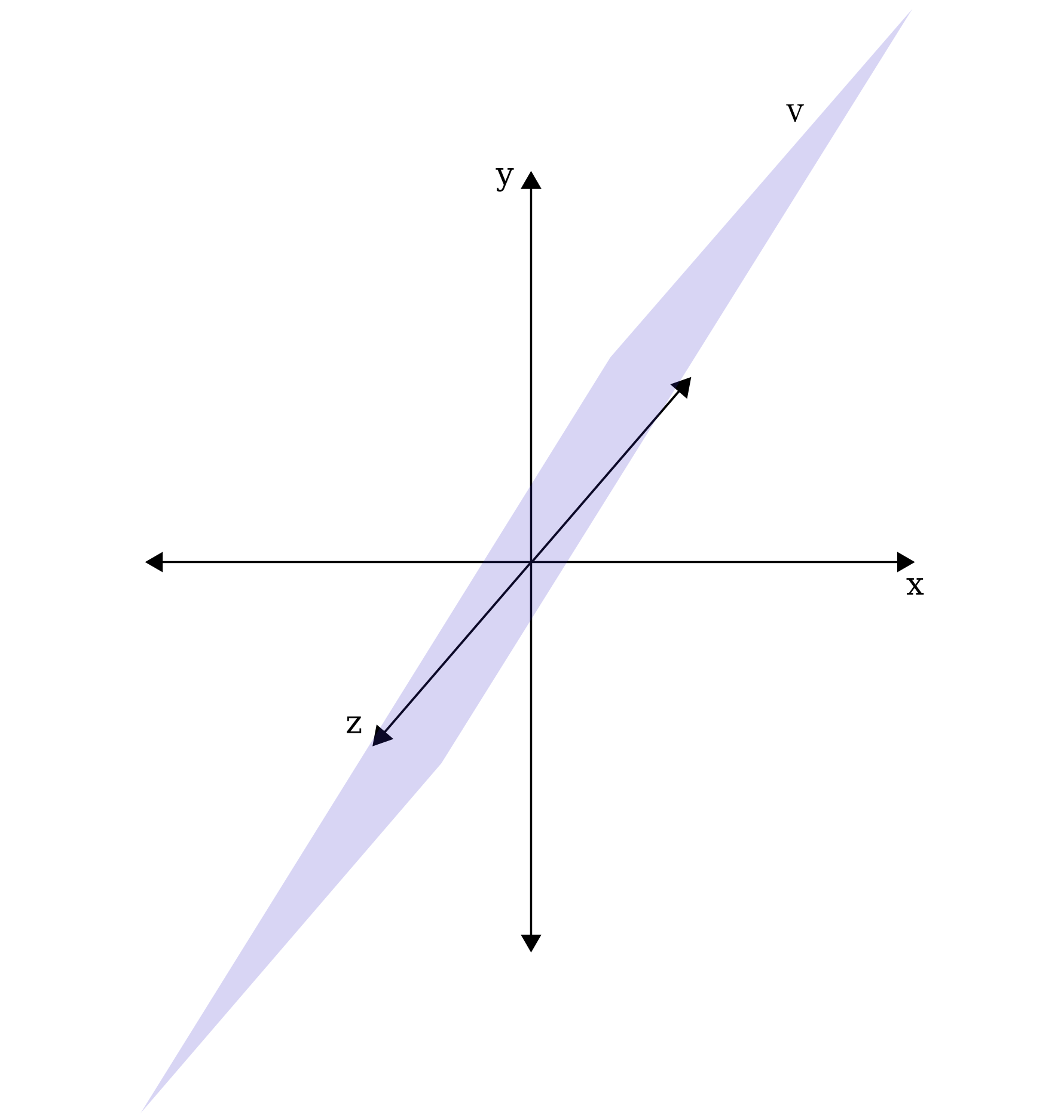
Consider some line V that passes through the origin in ℜ³ = {(a₁, a₂, a₃) ∣ a_i ∈ ℜ }. Do points in V form a vector space?

Do all points in V satisfy axioms ➀, ➃, ➄ and ➅?

Checking for axiom ➀

Since

If a, b and c are constants and parameter t is such that it is bounded by −∞ < t < +∞, then the equations x = x₀ + ta
y = y₀ + tb
z = z₀ + tc are called the parametric equation of a line with parameter t.

Thus, the line V through the origin (x₀ = 0, y₀ = 0, z₀ = 0) has a system equation of the form x = ta
y = tb
z = tc Consider two points on the line u = (u₁, u₂, u₃) and v = (v₁, v₂, v₃). Is the sum u + v = (u₁ + v₁, u₂ + v₂, u₃ + v₃) a point on the line V?

We know that the parametric equation of a line at point u is

u₁ = ta
u₂ = tb
u₃ = tc and at point v is v₁ = ta
v₂ = tb
v₃ = tc The parametric equation at a line at point u + v will be u₁ + v₁ = 2ta
u₂ + v₂ = 2tb
u₃ + v₃ = 2tc Depending upon the value of 2t the position of the point u + v will vary. But, this point will be on the line. Therefore, the above system is a parameteric equation of the point u + v on the line V. Hence, the closure law for addition, axiom ➀ is satisfied.

Checking for axiom ➃

Multiplying through the parameteric equation of a line at point u by 0 0 = 0 ⇒ u₁ = 0 in u₁ = ta
0 = 0 ⇒ u₂ = 0 in u₁ = tb
0 = 0 ⇒ u₃ = 0 in u₁ = tc we get the parameteric equation of a line at point 0 = (0, 0, 0). The point will lie on V because this point satisfies the parameteric equation of the line V through the origin x = ta
y = tb
z = tc Then, the parametric equation of a line at point u + 0 will be u₁ + 0 = ta + 0 ⇒ u₁ = ta
u₂ + 0 = tb + 0 ⇒ u₂ = tb
u₃ + 0 = tc + 0 ⇒ u₃ = tc the sum u + 0 = u.

Similarly, it can be shown that the sum 0 + u = u. Thus,

u + 0 = u = 0 + u = u Therefore, the law for adding zero vector, axiom ➃ is satisfied.

Checking for axiom ➄

Multiplying through the parametric equation of a line at point u by −1 −u₁ = −ta
−u₂ = −tb
−u₃ = −tc we get the parameteric equation of a line at point −u = (−u₁, −u₂, −u₃). The point will lie on V because this point satisfies the parameteric equation of the line V through the origin x = ta
y = tb
z = tc Then, the parameteric equation of a line at point u + (−u₁) will be u₁ + (−u₁) = ta − ta = 0
u₂ + (−u₂) = tb − tb = 0
u₃ + (−u₃) = tc − tc = 0 the parameteric equation of a line at the point 0 = (0, 0, 0). From above we know that this point lies on V. Thus, u + (−u) = u − u = 0 the negation law, axiom ➄ is satisfied.

Checking for axiom ➅

Multiplying through the parameteric equation of a line at point u by k ku₁ = kta
ku₂ = ktb
ku₃ = ktc we get the parameteric equation of a line at point ku = (ku₁, ku₂, ku₃). The point will lie on V because this point satisfies the parameteric equation of the line V through the origin x = ta
y = tb
z = tc Therefore, the closure law for multiplication, axiom ➅ is satisfied.

Since the above arguments show that points on the line V passing through the origin in ℜ³ satisfy all the ten axioms we can say that this set of points form a vector space.∎

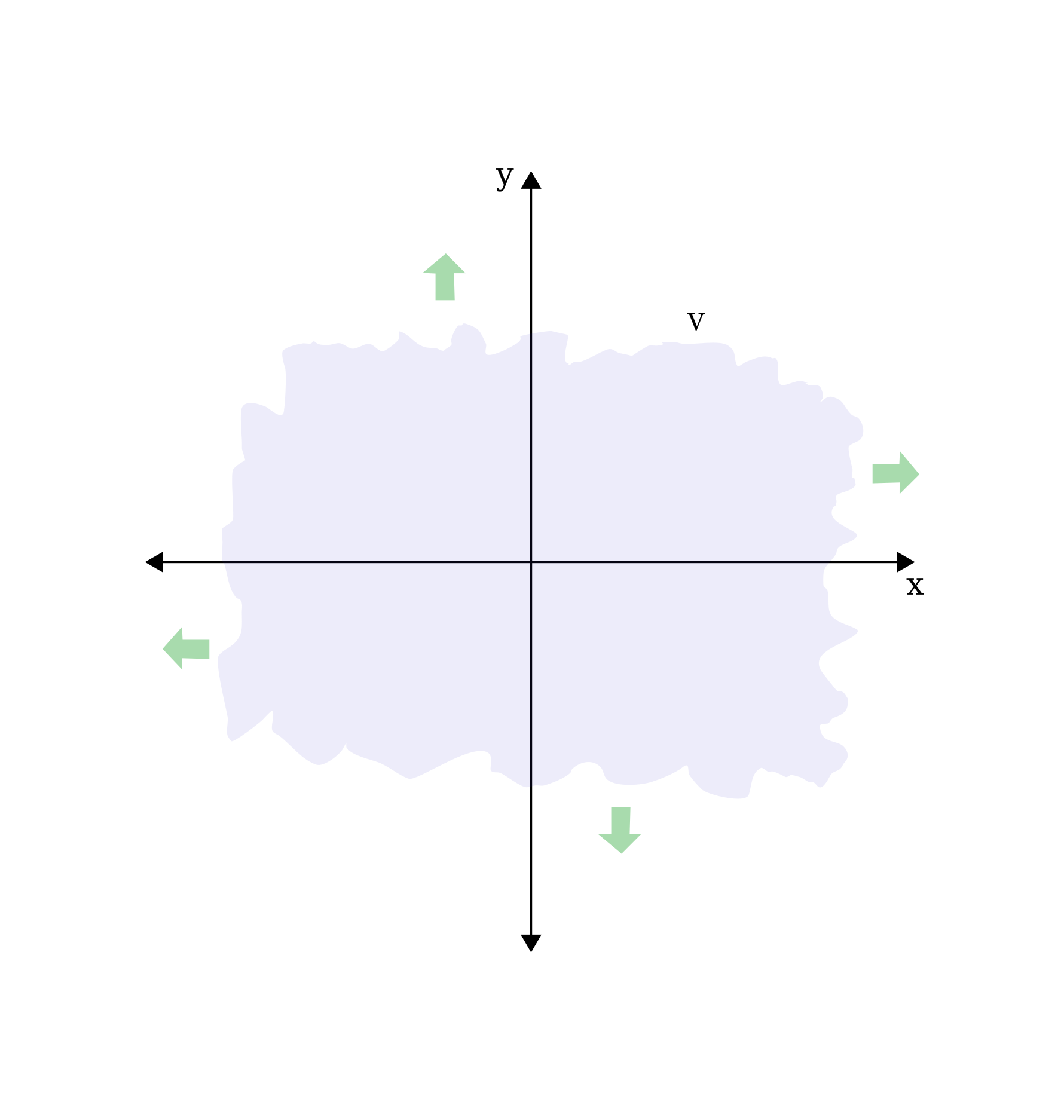
Consider the first quadrant of ℜ² as the plane V where ℜ² = {(a₁, a₂) ∣ a_i ∈ ℜ }. Do points in V form a vector space?

Since V is defined to be the set {(a₁, a₂) ∣ a_i ≥ 0} if u = (u₁, u₂) is a point in V then the point −u = (−u₁, −u₂) is not a point in V.

Thus, points on V do not satisfy axioms ➄, the negation law

u + (−u) = u − u = 0 because −u is not a point on V.

Since every point on V do not satisfy all the ten axioms we can say that this set of points do not form a vector space.∎

Consider the set of real valued function in ℜ as V² — functions whose values are on the the entire ℜ.. Does the set V form a vector space?

If u, v and w are functions in V u = u     whose value at x is     u(x) = u(x)
v = v     whose value at x is     v(x) = v(x)
w = w     whose value at x is     w(x) = w(x) such that operations defined are

function addition (u + v)x = u(x) + v(x) Adding the value of u at x = a to the value of v at x = a we obtain the value of u + v at x = a.

scalar multiplication of function (ku)x = ku(x) Multiply the value of u at x = a by the scalar k to get the value of ku at x = a

Thus, function u + v is an object in V and function ku is an object in V.

Therefore, axioms ➀ and ➅ — axioms that reflect definition of standard operations on ℜⁿ — are satisfied by all the functions in V.

Checking for axioms ➁ and ➂

Since (u + v)(a) = u(a) + v(a) and u(a), v(a) ∈ ℜ — (a, u(a)) and (a, v(a)) ∈ ℜ² — thus u(a) + v(a) = v(a) + u(a)
or
(u + v)(a) = (v + u)(a) Also, u(a) + (v + w)(a) = u(a) + [v(a) + w(a)]
u(a) + (v + w)(a) = [u(a) + v(a)] + w(a)
or
u(a) + (v + w)(a) = (u + v)(a) + w(a) Therefore, the commutative and associative laws for addition, axioms ➁ and ➂ are satisfied by all functions in V.

Checking for axioms ➃ and ➄

The zero function is the constant function whose value 0(x) is 0 for all x in ℜ 0 = 0 The negative of u is −u = −u whose value at x is −u(x) = −u(x)
Adding the values of 0 and u at x = a we get (0 + u)(a) = zero function at a + u(a) = 0 + u(a) = u(a) = u(a) Similarly, (u + 0)(a) = u(a) Therefore, the law of adding zero, axioms ➃ is satisfied.

Now, adding the values of u and −u at x = a we get

(u + −u)(a) = u(a) + −u(a) = u(a) − u(a) = 0 Also, (−u + u)(a) = 0 Therefore, the negation law, axioms ➄ is satisfied.

Checking for axioms ➆ and ➇

Since functions in V satisfy axioms ➀ and ➅ which corresponds to the definitions for standard operations consider the sum of two function u + v such that some scalar k multiplies the sum to obtain the function k(u + v). Then, for some x = a

If ku(a) is the scalar multiple at a and kv(a) is the scalar multiple at a then do their sum ku(a) + kv(a) equal k[u(a) + v(a)]?
If ku(a) is the scalar multiple at a and lu(a) is another scalar multiple at a then do their sum ku(a) + lu(a) equal (k + l)[u(a)]?

Axioms ➀ and ➅ tells us that the value of the k(u + v) function at x = a will be [k(u + v)](a) = k(u + v)(a)
[k(u + v)](a) = k[u(a) + v(a)] Since the values k, u(a) and v(a) are assumed to fall on the ℜ number line applying the distributive law of real numbers we know k[u(a) + v(a)] = ku(a) + kv(a) Thus, [k(u + v)](a) = ku(a) + kv(a)
k(u + v) = ku + kv for all x Therefore, the law for distributive multiplication over addition, axioms ➆ is satisfied.

If a scalar is the sum k + l then, from the scalar multiplication of functions we get

(k + l)u(a) = (k + l)u(a) Applying the law of multiplying real numbers by scalar sum we know (k + l)u(a) = ku(a) + lu(a) Thus, (k + l)u(a) = ku(a) + lu(a)
(k + l)u = ku + lu for all x Therefore, the law for multiplication by scalar sum, axioms ➇ is satisfied.

Checking for axioms ➈ and ➉

scalar multiple of function u by scalar l

If lu(a) is a scalar multiple at a then we obtain the function lu. The multiplication of this newly obtained function by the scalar k such that k[lu(a)] is a scalar multiple at a that yields k[lu(a)] = k[lu(a)] Since the values k, l and u(a) are assumed to fall on the ℜ number line applying the law of multiplication by product of real numbers we know k[lu(a)] = klu(a)
k[lu(a)] = (kl)u(a) Thus, k[lu(a)] = (kl)u Therefore, the multiplication by scalar product, axioms ➈ is satisfied.

For scalar multiple ku(a) at a if k = 1 we get 1u(a) as its scalar multiple at a thus,

1u(a) = 1 ⋅ u(a) Property of the number 1 tells us that 1 ⋅ u(a) = u(a) Thus, 1u(a) = u(a)
1u = u Therefore, the law of multiplication by one, axioms ➉ is satisfied.

Since the above arguments show that functions in V satisfy all the ten axioms we can say that this set of functons form a vector space.∎

Consider the set V contaning m × n matrices such that the matrix entries ∈ ℜ and the matrices can perform the operations, matrix addition and scalar multiplication. Then, $zero vector = [0 0 ... 0; 0 0 ... 0; ...; 0 0 ... 0]$ $u vector = [u11 u12 ... u1n; u21 u22 ... u2n; ...; um1 um2 ... umn]$ $v vector = [v11 v12 ... v1n; v21 v22 ... v2n; ...; vm1 vm2 ... vmn]$ Thus, for u $-u vector = -[u11 u12 ... u1n; u21 u22 ... u2n; ...; um1 um2 ... umn]$ Since

Assuming that the sizes of the matrices are such that the indicated operations can be performed, the following rules of matrix arithmetic are valid

ⓐ A + B = B + A
ⓑ A + (B + C) = (A + B) + C
ⓒ A(BC) = (AB)C
ⓓ A(B + C) = AB + AC
ⓔ (B + C)A = BA + CA
ⓕ A(B − C) = AB − AC
ⓖ (B − C)A = BA − CA
ⓗ a(B + C) = aB + aC
ⓘ a(B − C) = aB − aC
ⓙ (a + b)C = aC + bC
ⓚ (a − b)C = aC − bC
ⓛ (ab)C = a(bC)
ⓜ a(BC) = (aB)C = B(aC)

In general, given any sum or any product of matrices, pairs of parentheses can be inserted or deleted anywhere within the expression without affecting the end result.

Let, u = A, v = B, w = C
k = a, l = b, Then, ⓐ     becomes     u + v = v + u                            or     axiom ➁
ⓑ     becomes     u + (v + w) = (u + v) + w     or     axiom ➂
ⓗ     becomes     k(v + w) = kv + kw                or     axiom ➆
ⓙ     becomes     (k + l)w = kw + lw                 or     axiom ➇
ⓛ     becomes     (kl) = k(lw)                              or     axiom ➈ Therefore, axioms ➁, ➂, ➆, ➇ and ➈ are satisfied.

We know that 0, u, v and −u are objects in V whose matrix elements are in the real number line. We then find that

$vectors u + v = [u11+v11 u12+v12 ... u1n+v1n; u21+v21 u22+v22 ... u2n+v2n; ...; um1+vm1 um2+vm2 ... umn+vmn]$ Since every element of this matrix is in the real number line, the sum u + v will be an object in V. Therefore, axiom ➀ is satisfied.

For the axiom that deals with the rule of adding zero we can show that

$vectors 0 + u = [0+u11 0+u12 ... 0+u1n; 0+u21 0+u22 ... 0+u2n; ...; 0+um1 0+um2 ... 0+umn] = vector u$ and similarly for u + 0 = u. Thefore, axiom ➃ is satisfied.

For negation law we can show that

$vectors u + (-u) = [u11-u11 u12-u12 ... u1n-u1n; u21-u21 u22-u22 ... u2n-u2n; ...; um1-um1 um2-um2 ... umn-umn] = vector 0$ and similarly for &minuys;u + u = 0. Thefore, axiom ➄ is satisfied.

For any scalar multiplication operation

$scalar k times vector u = [k*u11 k*u12 ... k*u1n; k*u21 k*u22 ... k*u2n; ...; k*um1 k*um2 ... k*umn]$ all the matrix elements will lie on the real number line because any arbitrary scalar k was considered to lie on the real line. That is, the product ku will be an object in V. Thefore, axiom ➅ is satisfied.

Finally if k = 1

$scalar 1 times vector u = [1*u11 1*u12 ... 1*u1n; 1*u21 1*u22 ... 1*u2n; ...; 1*um1 1*um2 ... 1*umn] = vector u$ That is, 1u = u. Thefore, axiom ➉ is satisfied.

Since the above arguments show that any real matrices in V satisfy all the ten axioms we can say that this set of matrices form a vector space.∎

❺

Zero vector space

Given a finite vector space V consisting a single object denoted by 0 and 0 + 0 = 0
k0 = 0 for all k scalars then, V is a zero vector space.

Let V be a vector space, u a vector in V, and k a scalar; then 0u = 0
k0 = 0
(−1)u = −u
If ku = 0, then k = 0 or u = 0

Proof for 0u = 0

Since axiom ➇, multiplication by scalar sum, says

(k + l)u = ku + lu we can write (0 + 0)u = 0u + 0u But, 0 + 0 = 0 is a property of the number zero. Thus, 0u = 0u + 0u

Since axiom ➄, negation law, tells us that the negative of 0u is −0u, adding this to both sides of the expression we get

0u + (−0u) = (0u + 0u) + (−0u)

Axiom ➂, associate law for addition, says

u + (v + w) = (u + v) + w Therefore, our expression becomes 0u + (−0u) = 0u + [0u + (−0u)]

Axiom ➄, negation law, says

u + (−u) = u − u = 0 ⇒ 0u + (−0u) = 00 Thus, our expression gets further transformed to 00 = 0u + 0

From axiom ➃, adding zero, we know

u + 0 = 0 + u = u Hence, 00 = 0u + 0
becomes
00 = 0u∎

Proof for k0 = 0

Since axiom ➆, distributive multiplication over addition, says

k (u + v) = ku + kv we can write k(0 + 0) = k0 + k0

Axiom ➇, multiplication by scalar sum, says

(k + l)u = ku + lu Hence, (k + k)u = k0 + k0 Therefore, k(0 + 0) = k0 + k0
becomes
k(0 + 0) = (k + k)0 From property of numbers we know k + k = 2k, thus k(0 + 0) = (2k)0

From axiom ➃, adding zero, we know

u + 0 = 0 + u = u ⇒ 0 + 0 = 0 Hence, k(0 + 0) = (2k)0
becomes
k0 = (2k)0 Dividing both sides by k 0 = k0∎

Proof for (−1)u = −u

Proof for this can be achieved by demonstrating the negation law, axiom ➄, that is, show

u + (−1)u = 0 Consequently, (−1)u = −u

Since axiom ➉ tells us that 1u = u thus,

u + (−1)u = 1u + (−1)u Axiom ➇, multiplication by scalar sum, says (k + l)u = ku + lu Hence, u + (−1)u = 1u + (−1)u
become
u + (−1)u = (1 + −1)u But, property of numbers tell us that 1 + −1 = 0 therefore, 1u + (−1)u = 0u Since we proved that 0u = 0 1u + (−1)u = 0∎

Proof for if ku = 0 then 1) u = 0 or 2) k = 0

We proved k0 = 0 thus,

ku = 0
becomes
ku = k0 Therefore, u = 0∎¹

Axiom ➄, negation law, says

u + (−u) = u − u = 0 but ku = 0 is given. Hence u + (−1u) = 0
becomes
u + (−1u) = ku From axiom ➉ 1u = u thus the expression can be written as 1u + (−1u) = ku

Axiom ➇, multiplication by scalar sum, says

(k + l)u = ku + lu Hence, 1u + (−1u) = ku
become
[1 + (−1)]u = ku But, property of numbers tell us that 1 + −1 = 0 therefore, 0u = ku Therefore, k = 0∎²

❻

Subspace

The subset W of a vector space V is called a subspace of V if W is also a vector space under the standard operations (addition and scalar multiplication) defined on V.

If W ⊆ V vector space, then to verify W is a subspace of V one need to only test for axioms

➀ Closure law for addition
If u, v ∈ V, then u + v ∈ V
➃ Adding zero
There exists 0 ∈ V such that for all u ∈ V, u + 0 = 0 + u = u
0 is called the zero vector for V
➄ Negation law
For each u ∈ V there exists −u ∈ V such that u + (−u) = u − u = 0
and with commutative law for addition (Axiom ➁)
u + (−u) = (−u) + u = 0; −u is called negative of u
➅ Closure law for multiplication
If k is any real number scalar and u ∈ V, then ku ∈ V

because axioms ➁, ➂, ➆, ➇, ➈ and ➉ are inherited from V.

If W is a set of one or more vectors from a vector space V, then W is a subspace of V if and only if the following conditions hold.

W is closed under addition; If u and v are any vectors in W, then u + v is in W.
W is closed under scalar multiplication; If k is any scalar and u is any vectors in W, then ku is in W.

Let V be a vector space such that W ⊆ V and the two conditions holds

If u and v are any vectors in W, then u + v is in W.
If k is any scalar and u is any vectors in W, then ku is in W.

All objects in W satisfies axioms ➀ and ➅ because the two conditions reflect the axioms.

Since V is a vector space and W ⊆ V, then all objects in W automatically satisfies axioms ➁, ➂, ➆, ➇, ➈ and ➉.

Therefore, to prove W is a vector space and hence a subspace of V one only needs to check for axioms ➃ and ➄.

Let u be any vector in W. The second condition (above) tells us that for every scalar k, ku ∈ W. Then,

For k = 0, 0u = u is in W
For k = −1, (−1)u = −1u is in W

Thus, axioms ➃ and ➄ are satisfied.

Since all objects in W satisfy all the ten axioms and W is a subset of the vector space V we can say that the set W is a vector subspace.∎

Every vector space V has at least two subspaces; V itself is a subspace and the set {0}. The set {0} is called the zero subspace.

❼

Next:

Some Concepts of Linear Algebra (p:5) ➽

✪

Analytic properties of a vector provides deeper insight

Standard operations on ℜn

Generalizing Vector Space

Investigating if objects satisfy the set for generalized vectors

Checking for axiom ➀

Checking for axiom ➃

Checking for axiom ➄

Checking for axiom ➅

Checking for axiom ➀

Checking for axiom ➃

Checking for axiom ➄

Checking for axiom ➅

Checking for axioms ➁ and ➂

Checking for axioms ➃ and ➄

Checking for axioms ➆ and ➇

Checking for axioms ➈ and ➉

Zero vector space

Subspace

Standard operations on ℜⁿ